Kinetics

Collision theory, Maxwell–Boltzmann, rate equations, Arrhenius

Maxwell–Boltzmann distribution

• Shows the spread of molecular energies. Area under the curve = total number of molecules (constant).
• Higher T: peak shifts right and lower; many more molecules exceed E_a — rate rises steeply.
• Catalyst: provides an alternative route with lower E_a; the curve itself doesn't change, the E_a line moves left.

Rate equations (A-level year 2)

• Orders m, n come only from experiment, never from the equation's coefficients.
• The rate-determining step contains the species in the rate equation.

Arrhenius equation

A plot of ln k against 1/T is a straight line with gradient −E_a/R — how E_a is measured (required practical 3 uses this idea).

Try the Maxwell–Boltzmann simulation with the temperature slider.

3.1.9.1Finding orders from initial-rate data

3.1.9.1Concentration–time vs rate–concentration graphs

• [X]–time: zero order = straight line down; first order = curve with constant half-life; rate at any t = gradient of the tangent.
• rate–[X]: zero order = horizontal line; first order = straight line through the origin; second order = upward curve.

3.1.9.2Using the Arrhenius equation

• ln k = ln A − Ea/(RT): plot ln k (y) against 1/T (x) → gradient = −Ea/R, intercept = ln A.
• Gradient units: K. Multiply by −R (8.31 J K⁻¹ mol⁻¹) → Ea in J mol⁻¹; ÷1000 for kJ mol⁻¹.

Extended🎓 Beyond the standard course

• Molecularity ≠ order. Molecularity counts particles in one elementary step (always whole); order is experimental and can be zero or fractional. They coincide only for single-step reactions.
• Mechanism consistency test: NO₂ + CO → NO + CO₂ has rate = k[NO₂]². The slow step must use two NO₂ (NO₂ + NO₂ → NO₃ + NO), with CO mopping up NO₃ fast — CO absent from the rate law because it enters after the rate-determining step.
• Intermediates vs transition states: an intermediate sits in an energy dip (isolable in principle); a transition state is the summit — a bond-breaking/forming instant with no lifetime.
• Heterogeneous catalysis in three verbs: adsorb (reactants bond to surface, bonds weaken) → react (lower-Ea pathway) → desorb. Catalyst poisoning (Pb on catalytic converters) blocks the adsorption sites permanently.
• Autocatalysis (MnO₄⁻/C₂O₄²⁻) gives an S-shaped concentration–time curve: slow start, acceleration as the catalytic product accumulates, then substrate exhaustion.

Deep dive📚 The rest of the chapter, in full

What each change does to the Maxwell–Boltzmann curve

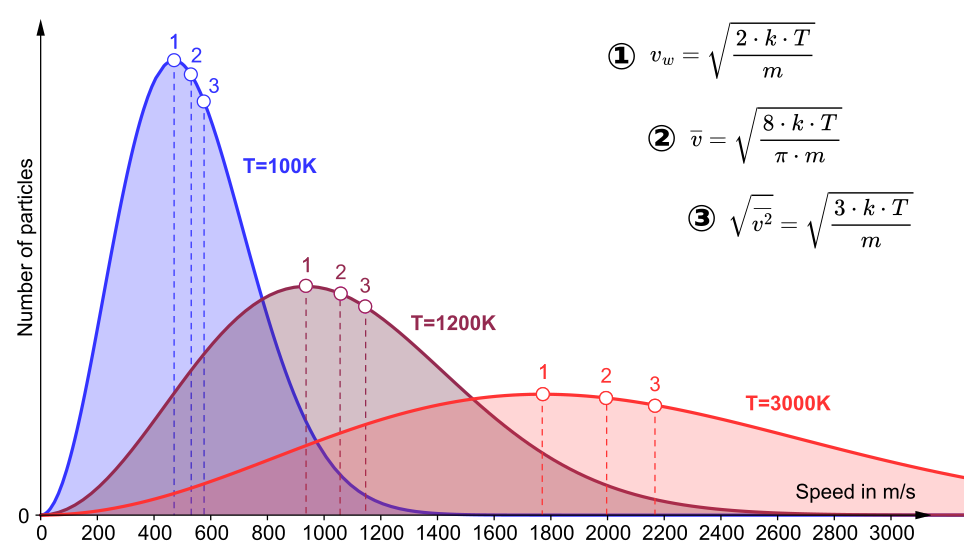
Never say a catalyst "lowers the activation energy of the reaction" — it provides an alternative route with a lower activation energy, and is unchanged at the end. Small temperature rises matter enormously: ~10 K roughly doubles rate because the high-energy tail grows exponentially.

Rate equations (Year 2 core)

rate = k[A]ᵐ[B]ⁿ — the orders m and n come only from experiment, never from the equation's coefficients. Total order = m + n. Units of k change with total order: mol dm⁻³ s⁻¹ ÷ (mol dm⁻³)ᵒʳᵈᵉʳ — first order gives s⁻¹, second order gives mol⁻¹ dm³ s⁻¹.

Arrhenius: getting Ea from experiment

k = Ae^(−Ea/RT), so ln k = ln A − Ea/RT. Plot ln k (or ln(1/t) from clock experiments) against 1/T: a straight line of gradient −Ea/R. With R = 8.31, a gradient of −5.4 × 10³ K gives Ea = 5.4 × 10³ × 8.31 ≈ 45 kJ mol⁻¹. Watch units — convert J to kJ at the end.

Mechanisms and the rate-determining step

The rate equation contains only species involved up to and including the slowest (rate-determining) step. If rate = k[(CH₃)₃CBr] with no [OH⁻], the slow step is the C–Br bond breaking alone (an SN1-style mechanism); OH⁻ attacks the carbocation in a later fast step. Reverse logic works too: propose mechanisms whose slow-step molecularity matches the orders.

Measuring rate in the lab

• Gas volume (syringe) or mass loss (open flask on a balance) against time — gradient of the tangent = rate at that moment; tangent at t = 0 gives the initial rate.
• Colorimetry for coloured species (e.g. the iodine or bromine concentration falling) — continuous, non-invasive.
• Clock methods (RP3/7): time to a fixed visible event; initial rate ∝ 1/t.

Mastery vault🏛 Every remaining spec point, banked

Reading the two graph families

• Concentration–time: zero order = straight line down (constant gradient); first order = curve with constant half-life (the definitive test — measure two successive half-lives, equal means first order); second order = curve with lengthening half-lives.
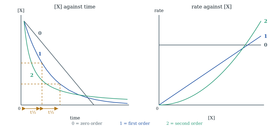
• Rate–concentration: zero order = horizontal line; first order = straight line through the origin (gradient = k); second order = upward curve (plot rate vs concentration² to straighten it).
• Know which graph you have been given before saying anything — mixing the families is the classic self-inflicted wound.

Initial-rates table, deduced properly

1→2: [X] ×2, rate ×4 → order 2 in X. 2→3: [Y] ×3, rate ×3 → order 1 in Y. rate = k[X]²[Y]; from expt 1, k = 2.0 × 10⁻⁴ ÷ (0.10² × 0.10) = 0.20 mol⁻² dm⁶ s⁻¹. Always finish with k's value AND units — half the marks sit there.

Arrhenius, both directions

The pre-exponential factor A represents collision frequency with correct orientation; e^(−Ea/RT) is the fraction of collisions with enough energy. Raising T leaves A almost alone but grows the exponential dramatically.

Mechanism–rate detective work

• The observed orders count how many of each species appear in steps up to and including the RDS. rate = k[NO]²[O₂]? A plausible mechanism: 2NO ⇌ N₂O₂ (fast), N₂O₂ + O₂ → 2NO₂ (slow) — the slow step's effective composition matches the rate law.
• Species appearing AFTER the RDS never feature in the rate equation; catalysts CAN feature (they act before/at the RDS); intermediates must not appear in the overall equation.
• Reverse test: proposed mechanisms whose slow step disagrees with observed orders are simply wrong — say so and why.